Home / DAIR Cloud / DAIR BoosterPack Catalogue / Flight Plan: Time-Series Prediction with Machine Learning / Sample Solution: Time-Series Prediction with Machine Learning

After January 17, 2025:

Screenshots should remain accurate, however where you are instructed to login to your DAIR account in AWS, you will be required to login to a personal AWS account.
Links to AWS CloudFormation scripts for the automated deployment of each sample application should remain intact and functional.
Links to GitHub repositories for downloading BoosterPack source code will remain valid as they are owned and sustained by the BoosterPack Builder (original creators of the open-source sample applications).

Time-Series Prediction with Machine Learning

If you haven’t already, please review the Bluwave-ai DAIR BoosterPack Flight Plan, Time-Series Prediction with Machine Learning, before implementing the Sample Solution below.

Introduction

The Time-Series Prediction with Machine Learning BoosterPack provides a deployable Sample Solution that allows users to observe and study the application of Machine Learning to solve the problem of developing models that provide predictions for Time-Series.

The purpose of this document is to describe the Sample Solution and how it demonstrates the use of advanced technologies. DAIR participants wishing to learn how to apply and adopt machine learning through artificial neural networks should find this content useful in deciding how, when, and if they’d like to follow similar approaches in their solutions.

This material is informed by the solutions that we develop at BluWave-ai to bring the power of AI to accelerating clean energy adoption. Our predictive-optimized control and transaction solutions increase the viability of the growing smart grids and micro-grids with renewable energy, storage, and electric vehicle charging.

Any terms identified with Capitalized Italics in this document are defined in the Glossary.

Problem Statement

The primary objective of time-series prediction is to develop models that provide plausible future values of a time-series, given past historical observation of the same and other time-series.

Time-series, i.e. a sequence of data taken at successive equal time-intervals, are prevalent in numerous applications in statistics, finance, meteorology, natural sciences, and engineering. Forecasting a time-series enables predictive actions that adjust system behaviour with respect to a plausible event in the future. The application opportunity domains are broad with the following as examples:

Energy optimization: AI-based smart grid optimization, particularly in the presence of highly variable and distributed renewables such as wind and solar.
Smart city: smart traffic control, security detection and dispatch, real-time transportation optimization.
Network and systems security: intrusion detection and control.
Infrastructure management: sensor-based deterioration detection, maintenance scheduling, depreciation and renewal optimization.
Real-time logistics: item placement, location, loading, and shipping optimization.
Medical applications: predicting future health risks, or recovery prediction, based on time series health diagnostics information.

Hallmarks of conventional time-series prediction techniques include: use of linear predictors, emphasis on problems with limited amount of training data, and efforts to determine distributional properties of residuals such that significance tests can be applied. These methods continue to be of great value.

The space of inference problems that can be practically addressed has recently expanded due to improvement in theory, increased availability of data, improved software ecosystem, and bigger usable hardware. These lead to practical advantages:

Handling larger amounts of data: longer historical observation periods exist and can be ingested together with parallel time-series that may contribute to prediction accuracy of the Target
Robust to data pre-processing: state-of-the-art machine learning techniques can handle mostly raw data, while conventional statistical inference models are potentially sensitive to bad historical data such as outliers or missing values. This is due to using non-linear vs. linear elements, and it being newly feasible to perform comprehensive model cross-validations.
Learning through a sequence: models such as Recurrent Neural Networks (RNNs) have attracted massive interest in time-series prediction due to their ability to exhibit temporal dynamic behaviour.
Automation friendly: machine learning techniques can be automated very effectively, and that facilitates continuous training and self-improvement.

Sample Solution

This Sample Solution showcases how machine learning can be used to address model generation and validation for time-series prediction.

Solution Overview

The solution includes two examples for training time-series predictors; one to predict Load (Model A) and another to predict wind speed (Model B). We use historical and meteorological data relevant to the respective problems. Each example begins with the raw data downloaded from the data source. The data then goes through a cleaning process that makes it more effective as input. Next, we prepare the data by removing and transforming existing features as necessary, and building new features based on the time-series nature of the data and/or any domain knowledge. At this point, if there are too many features for efficient training of the model, we perform feature selection. Then the data is divided into training and prediction sets, and the former is used to train our model, which is a neural network. An important part of training the model is optimizing its Hyper-parameters, which include both architectural and training settings. Lastly, with our trained model, we make predictions and evaluate goodness-of-fit with the prediction data. A machine learning model that has been well-built will provide plausible future values for the time-series of interest.

Solution Overview Diagram

The diagram below illustrates the structure of the Sample Solution.

Component Descriptions

Significant components used in the Sample Solution are summarized in the table below:

Component	Summary
Data source	Web source from which data is obtained.
Raw data	Time-series of historical and meteorological data relevant to the problem, downloaded from a public source.
“Clean”	Python script that pre-processes the data. Necessary steps include integrating data sets, removing or estimating missing entries, and scaling values.
Clean data	Data that has been “cleaned” from its raw format by undergoing pre-processing.
“Build”	Python script that builds new features, especially based on the time-series nature of the data.
Features	New potential inputs to the model, formulated from clean data along with existing data and features.
“Select”	Python script that implements feature selection algorithms which output a subset of given features.
Training data	The selected data and features which we want to use to train and optimize the neural network.
Prediction data	The selected data and features which we want to use to make predictions.
“Train”	Python script that implements a neural network, which learns how to predict the target quantity based on input data. TensorFlow and Keras libraries are both demoed.
Model	Artificial neural network that has undergone Supervised Learning.
“Predict”	Python script that makes predictions of the target quantity based on the trained neural network and prediction data.
Predictions	Plausible future values of the target quantity.

Technology Demonstration

This section guides you through a demonstration of machine learning model generation and validation with artificial neural networks (ANNs). Using machine learning is compelling because such models can learn continuously from a large volume of sequential data and are robust to input.

The demonstration will illustrate the training of two ANNs and their effectiveness as predictors for load and wind speed, respectively.

How to Deploy and Configure

If you’re a DAIR participant with access to a GPU, you can deploy this Sample Solution by following the instructions below. To complete these steps, you must already have or request an account on the DAIR OpenStack cloud with access to a GPU.

Log into the DAIR OpenStack cloud environment.
Navigate to Projects > Orchestration > Stacks, and click the + Launch Stack button

3. In the Select Template dialog, select URL as the Template Source and paste the following URL:

https://gpu-boosterpack-heat-templates.s3.ca-central-1.amazonaws.com/bluwave.yaml

into the Template URL field and then click Next.

In the Launch Stack dialog configure the application as shown in the figure below:

providing a name for the Stack,
a Password for the user (can be anything but not blank),
the Flavor/Instance Type of “v2.medium” and
Image of “Ubuntu 18.04 – 510”
then click the “Launch” button.

6. The sample application will now be deployed, taking roughly 5-10 minutes to complete. Post-provisioning scripts are also run automatically to set up the environment needed for the Sample Solution. Miniconda is installed, the repository containing the sample code is cloned, and the conda environments are created.

Once complete, you will need to get the private key created so that you can open a console (SSH) to the newly created GPU instance. To retrieve the private key, click on the Stack Name and scroll down until you find the private_key field and copy its contents to be used with your SSH client of choice.

Configuration and Application Launch

1. Once the application deployment is complete, initiate a console to the GPU instance via SSH using its external IP which can be found by navigating to Project > Compute > Instances as shown below.

2. To complete the Miniconda initialization, run the following commands:
/home/tsp/miniconda/bin/conda init exec bash

There are two examples packaged in the Sample Solution. Model A is an energy predictor implemented in Keras (with TensorFlow backend), while Model B is a weather predictor implemented in TensorFlow. Each takes between 15-20 minutes to train and validate their respective models.

3. To deploy Model A, run the following commands, waiting for each to complete before running the next command:
cd /home/tsp/time-series-prediction/energy-prediction conda activate energy-prediction make all
The first command takes you to the appropriate directory. The second command activates the appropriate Miniconda Python environment. The third command make all runs the Python scripts that prepare the data, train the model, and make predictions. (Here, ‘make’ refers to the software build automation tool.)

Alternately, to deploy Model B, run the following commands:
cd /home/tsp/time-series-prediction/weather-prediction conda activate weather-prediction make all
For Model A, you should observe the following output to the console:

Note: the loss values will vary due to the stochastic (random) elements of the model.

At the end, a quantification of the goodness-of-fit of the predictor is printed. This is compared to persistence (the naïve assumption), which simply predicts the current value for the next value. A time-series model is typically tested against this benchmark. The accuracy of this trained model is reflected in the low RMSE of the prediction (259.3146), relative to the RMSE of persistence (700.5231).

Additionally, visualizations of goodness-of-fit are generated and stored in /home/tsp/time-series-prediction/energy-prediction/reports/figures. First, all the prediction data is plotted:

For closer inspection, a subset of prediction data is also plotted:

As you can see, the model has learned to predict load very accurately.

For Model B, you should observe the following output to the console:

The model has learned to predict wind speed fairly accurately, and succeeds in beating persistence: the RMSE of the prediction is 4.6354, compared to the RMSE of persistence which is 4.9801.

The following plots are generated and stored in /home/tsp/time-series-prediction/weather-prediction/reports/figures:

Termination

Once you are finished exploring the Sample Solution, terminate the application to free up GPU resources for the DAIR community.

Navigate to Projects > Orchestration > Stacks, select the Stack and click Delete Stacks at the top (see figure below). This operation will delete the stack and the associated GPU instance. It should take less than 1 minute to complete.

Technology Considerations

Deployment Options

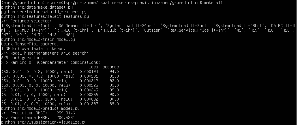
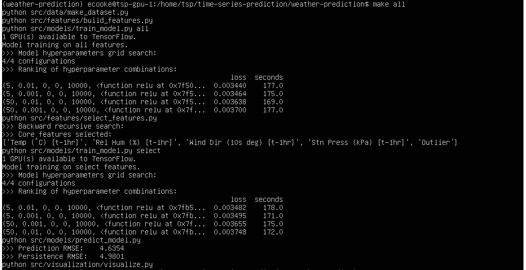
To improve predictor performance, you could increase the space over which the hyper-parameter grid search is done. This requires adding more values to the values in the dictionary in src/models/train_model.py, as in the Model A snippet shown below:

105 all_params = {'num_hidden': [75, 35],
106 'learn_rate': [0.001],
107 'lambda': [0, 0.01],
108 'dropout': [0, 0.2],
109 'num_epochs': [10000],
110 'activation': ['relu']}

Broadening the hyper-parameter search is done at the cost of time, since it requires exponentially more models to be trained and evaluated.

The Python scripts that constitute the Sample Solution are only supported on Linux systems.

Technology Alternatives

One of the key technology decisions in this solution was to use an ANN as the machine learning model, and we built a multi-layer Perceptron (MLP) with Back-propagation. This was done for the sake of simplicity, as a perceptron is the most basic form of an ANN. However, a strong alternative is a recurrent neural network (RNN), as it can exhibit temporal dynamic behaviour relevant to time-series. Long short-term memory (LSTM) networks are very powerful RNNs and should be explored to achieve better performance for more complex problems.

Artificial neural networks need not be used. With time-series prediction you almost always face a regression problem, where your prediction is a real number. Other models such as linear regression or polynomial regression can be very effective. You may consider these methods if you have a relatively small data-set, or depend heavily on the interpretability of the model, since ANNs are inferior in these areas.

In terms of software development, we chose to use the Keras and TensorFlow libraries in Python to implement the model. This decision was based on the popularity of Python and these two libraries, but also because the Python + Keras is a great combination for beginners. Alternative machine learning libraries in Python are Theano, PyTorch, and scikit-learn. Alternatives in C++ are Microsoft CNTK and Caffe, and in C, Torch. These all generally yield improvements in speed over Python implementations.