Flight Plan: Time-Series Prediction with Machine Learning

Flight Plan Overview

For data-driven companies needing to improve prediction for their time-series data, the Sample Solution demonstrates how machine learning is used to create highly accurate predictors. Unlike conventional statistical inference techniques, this Sample Solution achieves models that can learn continuously from a large volume of sequential data and are robust to input.

Please see the Time-Series Prediction with Machine Learning: Sample Solution for more information on how the Sample Solution works.

The Sample Solution showcases two technologies: machine learning and time-series prediction methods, described in subsequent sections. This BoosterPack features machine learning and demonstrates its application to solving time-series prediction problems.

Flight Plan: Machine Learning

Machine learning is the field of computer science that develops algorithms in which the computer (i.e. machine) is not explicitly programmed, but rather observes patterns in data (i.e. learns) to build models that make decisions or predictions. We will concentrate on supervised learning, in which the algorithm is given a data-set of inputs and desired outputs. During the learning process, we feed this data to the model, and the algorithm that we have implemented builds a model accordingly. The goal is to produce a trained model that, given input, can predict reasonable output values and provide valuable forecasts.

We chose to build artificial neural networks (ANNs) in the Sample Solution because of the remarkable results that have been achieved with them in the field of machine learning, and their subsequent popularity. We implemented a feed-forward MLP network with back-propagation. Review Chapter One of “Neural Networks and Deep Learning” for a complete explanation of how ANNs operate, and Chapter Two to understand the math behind back-propagation. For an intuition of how neural networks behave, try exploring the TensorFlow playground.

Resources

Please see the sections below for resources on machine learning.

Access to the Sample Solution source code will be a helpful learning resource. For both the energy-prediction or weather-prediction examples, review the contents of the /notebooks, /src/data, /src/features, and /src/models folders.

Tutorials

The table below provides a non-comprehensive list of links to tutorials the author has found to be most useful.

Documentation

Please see the table below for a set of documentation resources for Time-Series Prediction with Machine Learning.

Support

No additional support resources are applicable here.

Best Practices

• Standardized structure:When setting up your project directory structure, we recommend following the structure proposed in Cookiecutter Data Science. A standardized structure makes it easier for someone else to understand your code and analysis, and easier for you to jump back into your code months or years later. Besides, nothing is binding, so you still have flexibility with your work. The Sample Solution illustrates one implementation of this structure, as does this tutorial/example. We recommend you follow the Cookiecutter structure for all your data science projects.
• Virtual environments:A crucial part of data science is making sure your work is reproducible. Virtual environments help by giving you a blank environment every time you start a new project and capturing all the libraries and versions installed along the way. Therefore, your project environment is kept independent from the rest of your system and can be exported for users on other machines to recreate. Anaconda/Miniconda and virtualenv both support the creation of virtual environments. We recommend you create a virtual environment for every project you begin.

Tips and Traps

• Tip:there are some significant differences in doing machine learning with time-series than with non-sequenced data. Be careful applying standard machine learning techniques that you read about, if they are not given in the context of time-series modeling! Some traps are:
  • Dropping entries in data pre-processing. With non-sequenced data, you can choose to drop entries that are outliers or have missing values. But with time-series it is crucial that the data is taken at successive equal time-intervals. Thus, nothing can be dropped.
  • Caution with shuffling during training. Some libraries may shuffle your data, which ruins the sequential input of your time-series to the model. For example, the default behaviour of fit() in Keras shuffles the data in between each epoch. Make sure you turn this off.
  • When dividing the data into the training, validation, and test sets, the sequential nature of the data must be maintained; otherwise, future knowledge “leaks” into the past. The validation data must chronologically follow the training data, and the test data must follow the validation data (and thus is always the most recent). This also means that traditional cross-validation is not allowed, as it violates time sequencing. You may consider nested cross-validation
• Tip: rule-of-thumb settings for model hyper-parameters. Some hyper-parameters relate to the architecture of the model, such as number of hidden layers, number of nodes in the hidden layer(s), and the activation function(s) at each layer. Other hyper-parameters affect the learning process, such as the optimizer, learning rate, regularization weight, dropout frequency, objective function, performance metric, and number of epochs to train. Here are some rules-of-thumb:
  • Number of hidden layers: one hidden layer is usually sufficient.
  • Number of hidden nodes: proportional to the perceived complexity of the system being modeled. Start in the range of 1/10 the number of inputs.
  • Activation function: we recommend ReLu, which is standard because it can avoid the vanishing gradient problem suffered by sigmoid and tanh.
  • Optimizer: we recommend Adam, which has been shown to work well.
  • Learning rate: this is the hyper-parameter that will affect model performance the most. The standard learning rate for the Adam optimizer is 0.001, but experiment with neighbouring powers of 10.
  • Regularization weight: start with 0.01 and experiment with neighbouring powers of 10, depending on how much the model is over-fitting.
  • Dropout frequency: experiment with values from 0 to 30%, depending on how much the model is over-fitting.
  • Objective function: mean squared error (MSE) or mean average error (MAE) are both standard for regression problems.
  • Performance metric: mean squared error (MSE) or mean average error (MAE) are sensible metrics for time-series regression. You can choose the same metric as used for the objective function.
  • Number of epochs: observe your learning curves to see how many epochs it takes for them to plateau. When training without batching, as we do in the reference solution, start in the range of 1,000 to 10,000.
• Tip: deep learning will almost always benefit from the use of a GPU. The advantage of a GPU is its efficiency in doing matrix multiplication, which is how weights are propagated throughout a neural network. This is especially beneficial as you use larger batch sizes, or in our case do not use batching at all but feed all your training data in at once. The decision to use multiple GPUs needs more consideration.
• Tip: expect some randomness in your model results. ANNs have an element of randomness in the initialization of model weights. Hence you can expect your numbers to be slightly different each time you train your model, even on the same data-set.

Flight Plan: Time-Series Prediction Methods

In the Sample Solution, we apply machine learning techniques to create a time-series predictor. With time-series data, we are especially interested in its time-dependent behaviour, such as trend and seasonality. For a quick introduction to those terms, visit Section 2.3 of “Forecasting: Principles and Practice.” Below is an example of time-series data:

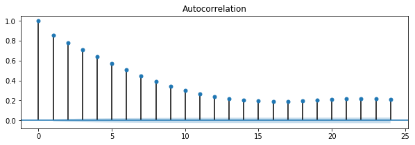
The core strategy is to introduce features that explicitly communicate information implicit in the time-series. The most significant of these is the addition of “lag” features, which capture the predictive power in the sequential nature of our observed data. For each time-step (t), experience tells us that the time-step immediately prior, (t-1), has strong predictive value. To quantify this, we inspect an auto-correlation plot to see which time lags are most strongly correlated with the present value. The x-axis marks the time-step lag and the y-axis marks correlation values. The auto-correlation plot captures the tendency for all time-steps t.

Tutorials

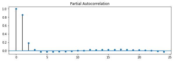
As expected, we see that the lags closest to the value are the most highly correlated. In particular, the value at lag 0 is perfectly correlated (correlation value 1.0), because the value is being measured against itself. However, there is a sequential dependency to be considered. Though (t-2) looks highly correlated with (t), this might merely be a propagation of the correlation in (t-1). Therefore, it is helpful also to inspect the partial auto-correlation plot, which removes these dependencies to give us a better idea of which lag features are essential.

We see that the correlation between (t) and (t-2) is now reduced from 0.8 to 0.2, and all lags beyond (t-2) have no strong independent correlation with the present time. Auto-correlation and partial auto-correlation plots can also make us aware of seasonality in the data. Seeing a strong correlation between (t) and (t-24), for example, indicates that the data has daily seasonality.

Another way to communicate time-dependencies as features is to perform “one hot encoding.” This is the translation of a categorical variable, with x categories, into x binary features. With time-dependent processes, information such as hour of the day, day of the week, or month of the year are all potentially relevant features to encode.

Lastly, we borrow the concept of time-differencing from conventional time-series forecasting techniques. This approach is to remove rather than represent trend and seasonality, in hopes of making the data easier to model. Section 8.1 of “Forecasting: Principles and Practice” provides a good description of the technique, and you can use differencing to transform your data or build new features. We do not use differencing in our models because the other methods prove sufficient.

Resources

Please see sections below for resources on time-series prediction methods.

Access to the Sample Solution source code will be a helpful learning resource. For both the energy-prediction or weather-prediction examples, review the contents of the /data, /notebooks, /src/data, and /src/features folders.

Tutorials

The table below provides a non-comprehensive list of links to tutorials the author has found to be most useful.

Documentation

Please see the table below for a set of documentation resources for Time-Series Prediction with Machine Learning.

Support

No additional support resources are applicable here.

Best Practices

• Notebooks:The first step after loading your data is to explore its characteristics. In Python, Jupyter notebooks are handy for this task because of their interactivity. For machine learning, decisions about data pre-processing and feature building and selection should be supported by work done in notebooks. We recommend you use notebooks to save and communicate this data exploration process.

Tips and Traps

• Trap: be cautious with accidentally leaking data. This can arise when:
  • Future timestamps leak into the past. Make sure your machine learning algorithm is never allowed to “see into the future.” This also includes the present, so that you cannot include any data from the time for which you are making your prediction. Concretely, when making a prediction at time t, the model may not have already ingested data from time t or later.
  • Testing (or validation) data leaks into training data. The advantage of segregating data into training, validation, and test sets is lost when the optimization phase can access validation data, or the training phase can access test data.
  • Target variable leaks into the features. This might happen implicitly if you mistakenly build features based off the target. For example, when constructing a binary outlier feature, counting outliers of the target would constitute data leakage.
• Tip: aim to beat persistence. The most naïve time-series predictor, “persistence”, simply predicts the current value for the next value. This model can unintelligently achieve impressively low error scores. Whenever developing a time-series predictor, benchmark the performance of your model against persistence. This will also prevent you from the trap of trying to predict a quantity that is the product of a random walk, as this author warns against. If your model cannot beat persistence, it may be evidence that your target quantity is quite literally unpredictable.